Satellite imagery processing for deep learning application
Introduction
Remember the pain you go through working with very cloudy satellite images? Where lowering the cloud percentage would mean that you will have little or no images to work with? Moreso painful and frustrating when you build a very good deep-learning model only to realize that the inference component is extra challenging because the single image to predict with is almost always cloudy. This is even more prevalent when you are working with optical imageries such as Sentinel-2.
A recent project to develop a deep learning model to predict and estimate cropland area from freely available optical satellites further highlighted the need to design a solution.
In this blog post, I will share with you how to identify cloudy pixels and replace them with alternative satellite images. Overall, the combination of high spatial resolution, multi-spectral capabilities, frequent coverage, open data access, and cloud cover monitoring makes Sentinel-2 a preferred choice for agriculture and land use applications, facilitating more informed decision-making and sustainable land management practices. Despite the advantages of using Sentinel-2, this optical imagery suffers in areas (locations) where there are a lot of cloud covers.
Image acquisition
For this tutorial, the ROI will be located in Rwanda. Rwanda’s tropical climate, topography, proximity to the Intertropical Convergence Zone(ITCZ), seasonal variation, and potential impacts of climate change contribute to the prevalence of cloud cover in the region making it ideal for this tutorial. We use Sentinelhub to access freely available Sentinel-2 and Landsat 8 and(or) 9. To register for Sentinelhub, head over here, and create a client ID and client secret for your account.
Now, in the code environment, import the necessary modules.
from sentinelsat import SentinelAPI
from datetime import date

from shapely.ops import unary_union

import geopandas as gpd
from shapely.geometry import shape
from sentinelhub import BBox, CRS, DataCollection, SentinelHubRequest, MimeType, SHConfig
import rasterio
import numpy as np
import matplotlib.pyplot as plt
from rasterio.plot import show
from matplotlib.patches import Patch
from rasterio.plot import show
import os
import fiona
from rasterio import mask
Set your Sentinel Hub credentials
config = SHConfig()
config.sh_client_id = 'Add your Sentinel Hub instance ID'
config.sh_client_secret = 'Add your Sentinel Hub client secret'
Next, we set the date range for which the images will be downloaded, and the location over which the image will be downloaded. We set the cloud_cover to 0.25. In general, this value ensures we retain only images having 0.25 as maximum cloud cover.
Set the path to your shapefile
shapefile_path = "/path/to/shapefile.shp/"

#Set the date range for the Sentinel-2 image search
start_date = date(2024, 1, 1)
max_cloud_cover = 0.25

end_date = date(2024, 3, 30)
#image size to be downloaded
image_size = (512, 512)
# Define the mean and standard deviation values for normalization
mean = [0.485, 0.456, 0.406]
std = [0.229, 0.224, 0.225]
Set up Sentinel Hub API including the bands to download
#Sentinel 2 bands to be downloaded
bands = ["B01", "B02", "B03", "B04", "B05", "B06", "B07", "B08", "B8A", "B09", "SCL", "B11", "B12","SCL"]

#Sentinel 1 bands to be downloaded
bands_s1 = ['VV', 'VH']
#Landsat 8,9 bands to be downloaded
l_band = ["B02", "B03", "B04","B05"]

api = SentinelAPI(config.sh_client_id, config.sh_client_secret, 'https://scihub.copernicus.eu/dhus')
evalscript = """
//VERSION=3
function setup() {
    return {
        input: ["B01", "B02", "B03", "B04", "B05", "B06", "B07", "B08", "B8A", "B09", "B11", "B12","SCL"],
        output: [
            { id: "B01", bands: 1, sampleType: SampleType.AUTO },
            { id: "B02", bands: 1, sampleType: SampleType.AUTO },
            { id: "B03", bands: 1, sampleType: SampleType.AUTO },
            { id: "B04", bands: 1, sampleType: SampleType.AUTO },
            { id: "B05", bands: 1, sampleType: SampleType.AUTO },
            { id: "B06", bands: 1, sampleType: SampleType.AUTO },
            { id: "B07", bands: 1, sampleType: SampleType.AUTO },
            { id: "B08", bands: 1, sampleType: SampleType.AUTO },
            { id: "B8A", bands: 1, sampleType: SampleType.AUTO },
            { id: "B09", bands: 1, sampleType: SampleType.AUTO },
            { id: "B11", bands: 1, sampleType: SampleType.AUTO },
            { id: "B12", bands: 1, sampleType: SampleType.AUTO },
            { id: "RGB", bands: 3, sampleType: SampleType.AUTO },
            { id: "RGBN", bands: 4, sampleType: SampleType.AUTO },
            { id: "TCI", bands: 3, sampleType: SampleType.AUTO },
            { id: "NDVI", bands: 1, sampleType: SampleType.FLOAT32 },  // NDVI band
            { id: "SAVI", bands: 3, sampleType: SampleType.FLOAT32 },
            { id: "SCL", bands: 3, sampleType: SampleType.FLOAT32 },

        ]
    };
}
# Define any vegetation indices you are interested in
function evaluatePixel(samples, scenes, inputMetadata, customData, outputMetadata) {
    ndvi = (samples.B08 - samples.B04) / (samples.B08 + samples.B04);

    // Calculate SAVI
    L = 0.5;  // Soil brightness correction factor (adjust as needed)
    savi = ((samples.B08 - samples.B04) / (samples.B08 + samples.B04 + L)) * (1 + L);

    return {
        B01: [samples.B01],
        B02: [samples.B02],
        B03: [samples.B03],
        B04: [samples.B04],
        B05: [samples.B05],
        B06: [samples.B06],
        B07: [samples.B07],
        B08: [samples.B08],
        B8A: [samples.B8A],
        B09: [samples.B09],
        B11: [samples.B11],
        B12: [samples.B12],
        RGB: [2.5*samples.B04, 2.5*samples.B03, 2.5*samples.B02],
        RGBN: [samples.B04, samples.B03, samples.B02, samples.B08],
        TCI: [3*samples.B04, 3*samples.B03, 3*samples.B02],
        NDVI: [ndvi],
        SAVI: [savi],
        SCL: [samples.SCL],
    };
}
"""
api = SentinelAPI(config.sh_client_id, config.sh_client_secret, 'https://scihub.copernicus.eu/dhus')
evalscript_s1 = """
//VERSION=3
function setup() {
    return {
        input: ["VV", "VH"],
        output: [
            { id: "VV", bands: 1, sampleType: SampleType.AUTO },
            { id: "VH", bands: 1, sampleType: SampleType.AUTO },
            { id: "RGB", bands: 3, sampleType: SampleType.AUTO }

        ],
        visualization: {
            bands: ["VV", "VH"],
            min: [-25,-25], // Adjust these values based on your data distribution
            max: [5,5], // Adjust these values based on your data distribution
        }
    };
}

function evaluatePixel(samples, scenes, inputMetadata, customData, outputMetadata) {
    // Adjust the coefficients for a natural color representation
    ratio = samples.VH-samples.VV
    rgb_ratio = samples.VH+ samples.VV+ratio
    red = samples.VH;
    green = samples.VV;
    blue = rgb_ratio;
    return {
        VH: [red],
        VV: [green],
        RGB: [red, green, blue]
    };
}
"""

api = SentinelAPI(config.sh_client_id, config.sh_client_secret, 'https://scihub.copernicus.eu/dhus')
evalscript_l8 = """
//VERSION=3
function setup() {
    return {
        input: ["B02", "B03", "B04","B05"], // Bands for true color and NIR
        output: [
            { id: "rgb", bands: 3,  sampleType: SampleType.AUTO}, // True color RGB
            { id: "ndvi", bands: 3,  sampleType: SampleType.AUTO} // NDVI
        ]

    };
}

function evaluatePixel(samples, scenes, inputMetadata, customData, outputMetadata) {
    // Calculate NDVI
        ndvi = (samples.B05 - samples.B04) / (samples.B05 + samples.B04);

    // Return true color RGB and NDVI values
    return {
        rgb: [2.5*samples.B04, 2.5*samples.B03, 2.5*samples.B02], // True color RGB
        ndvi: [ndvi] // NDVI
    };
}
Define python function to download the satellite images which makes a call to the Sentinel Hub APIs defined above
# Function to download Sentinel-2 images using sentinelhub
def download_sentinel_images(api, shapefile_path, start_date, end_date, output_folder):
    # Load the shapefile into a GeoDataFrame
    gdf = gpd.read_file(shapefile_path)
    gdf = gdf.set_geometry('geometry')

    # Set the common CRS for both the shapefile and tiles
    common_crs = 'EPSG:32736'
    # Read the shapefile into a GeoDataFrame
    gdf = gpd.read_file(shapefile_path)

    # Calculate the area of each polygon in square meters
    target_crs = 'EPSG:32736'
    gdf = gdf.to_crs(target_crs)

    gdf['area_m2'] = gdf['geometry'].area

    # Calculate the bounding box of the union of all geometries in the shapefile
    shapefile_union = unary_union(gdf['geometry'])
    bbox = BBox(bbox=shape(shapefile_union).bounds, crs=CRS(common_crs))

    # Iterate over polygons
    for idx, row in gdf.iterrows():
        polygon = row['geometry']


        request = SentinelHubRequest(
            data_folder=os.path.join(output_folder, 'sentinel2'),
            evalscript=evalscript,
            input_data=[
                SentinelHubRequest.input_data(
                    data_collection=DataCollection.SENTINEL2_L2A,
                    time_interval=(start_date, end_date),
                    mosaicking_order='mostRecent',
                    maxcc=max_cloud_cover
                )
            ],
            responses=[
                SentinelHubRequest.output_response('RGB', MimeType.TIFF),
                SentinelHubRequest.output_response('SCL', MimeType.TIFF)
            ],
            bbox=bbox,
            size=image_size,
            config=config
        )

        try:
            request.save_data()


            print(f"Data saved successfully for polygon {idx}!")
        except Exception as e:
            print(f"Error saving data for polygon {idx}: {e}")


def download_landsat_images(api, shapefile_path, start_date, end_date, output_folder):
    # Load the shapefile into a GeoDataFrame
    gdf = gpd.read_file(shapefile_path)
    gdf = gdf.set_geometry('geometry')


    # Set the common CRS for both the shapefile and tiles
    common_crs = 'EPSG:32736'
    # Read the shapefile into a GeoDataFrame
    gdf = gpd.read_file(shapefile_path)

    # Calculate the area of each polygon in square meters
    target_crs = 'EPSG:32736'
    gdf = gdf.to_crs(target_crs)

    gdf['area_m2'] = gdf['geometry'].area

    # Calculate the bounding box of the union of all geometries in the shapefile
    shapefile_union = unary_union(gdf['geometry'])
    bbox = BBox(bbox=shape(shapefile_union).bounds, crs=CRS(common_crs))

    # Iterate over polygons
    for idx, row in gdf.iterrows():
        polygon = row['geometry']


        request = SentinelHubRequest(
            data_folder=os.path.join(output_folder, 'landsat'),
            evalscript=evalscript_l8,
            input_data=[
                SentinelHubRequest.input_data(
                    data_collection=DataCollection.LANDSAT_OT_L1,
                    time_interval=(start_date, end_date),
                    mosaicking_order='mostRecent',
                    maxcc=max_cloud_cover

                )
            ],
            responses=[
                SentinelHubRequest.output_response('rgb', MimeType.TIFF),
                SentinelHubRequest.output_response('ndvi', MimeType.TIFF)
            ],
            bbox=bbox,
            size=image_size,
            config=config
        )

        try:
            request.save_data()


            print(f"Data saved successfully for polygon {idx}!")
        except Exception as e:
            print(f"Error saving data for polygon {idx}: {e}")
We may want to create patches from very large shapefiles. To achieve this, the below code block is helpful
def preprocess_patch(patch):
    # Convert to RGB format
    patch_rgb = np.transpose(patch, (1, 2, 0))
    # Convert to PIL Image
    patch_image = Image.fromarray((patch_rgb * 255).astype(np.uint8))
    # Resize the image to match the model's input size
    patch_image = patch_image.resize((512, 512))
    # Apply transformations
    transform = transforms.Compose([
        transforms.ToTensor(),
        transforms.Normalize(mean, std)
    ])
    # Convert to PyTorch tensor
    patch_tensor = transform(patch_image)
    # Add a batch dimension
    patch_tensor = patch_tensor.unsqueeze(0)
    return patch_tensor

def create_patches_from_single_image(image_path, patch_size=512):
    num_patches_total = 0
    total_predictions = np.zeros((1, 1, 512, 512))

    try:
        with rasterio.open(image_path) as src:
            num_patches = 0

            for i in range(0, src.width, patch_size):
                for j in range(0, src.height, patch_size):
                    window = rasterio.windows.Window(i, j, patch_size, patch_size)
                    patch = src.read(window=window)

                    processed_patch = preprocess_patch(patch)

                    # Make predictions on the processed patch
                    with torch.no_grad():
                        predictions_patch = loaded_model(processed_patch.to(device))
                        predictions_patch = torch.sigmoid(predictions_patch)
                        predictions_patch = predictions_patch.cpu().numpy()

                        # Accumulate the predictions
                        total_predictions += predictions_patch

                    # For now, just print the patch information
                    print(f"Patch {num_patches + 1}: {window}")

                    num_patches += 1
                    num_patches_total += 1


    except rasterio.errors.RasterioIOError as e:
        print(f"Error opening the image at {image_path}: {e}")

    return num_patches_total
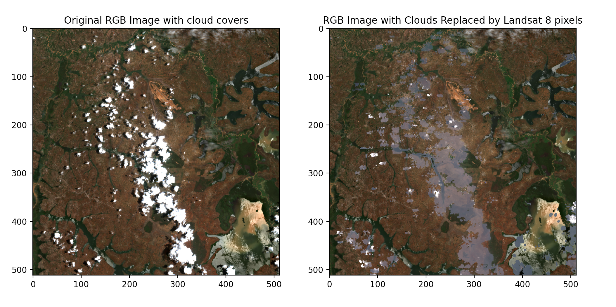
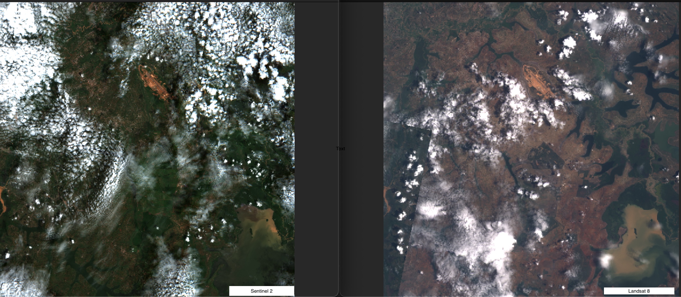
Executing the above blocks of code will give us the most recent Sentinel 2 image on the left and the Landsat 8 image on the left.
Goal
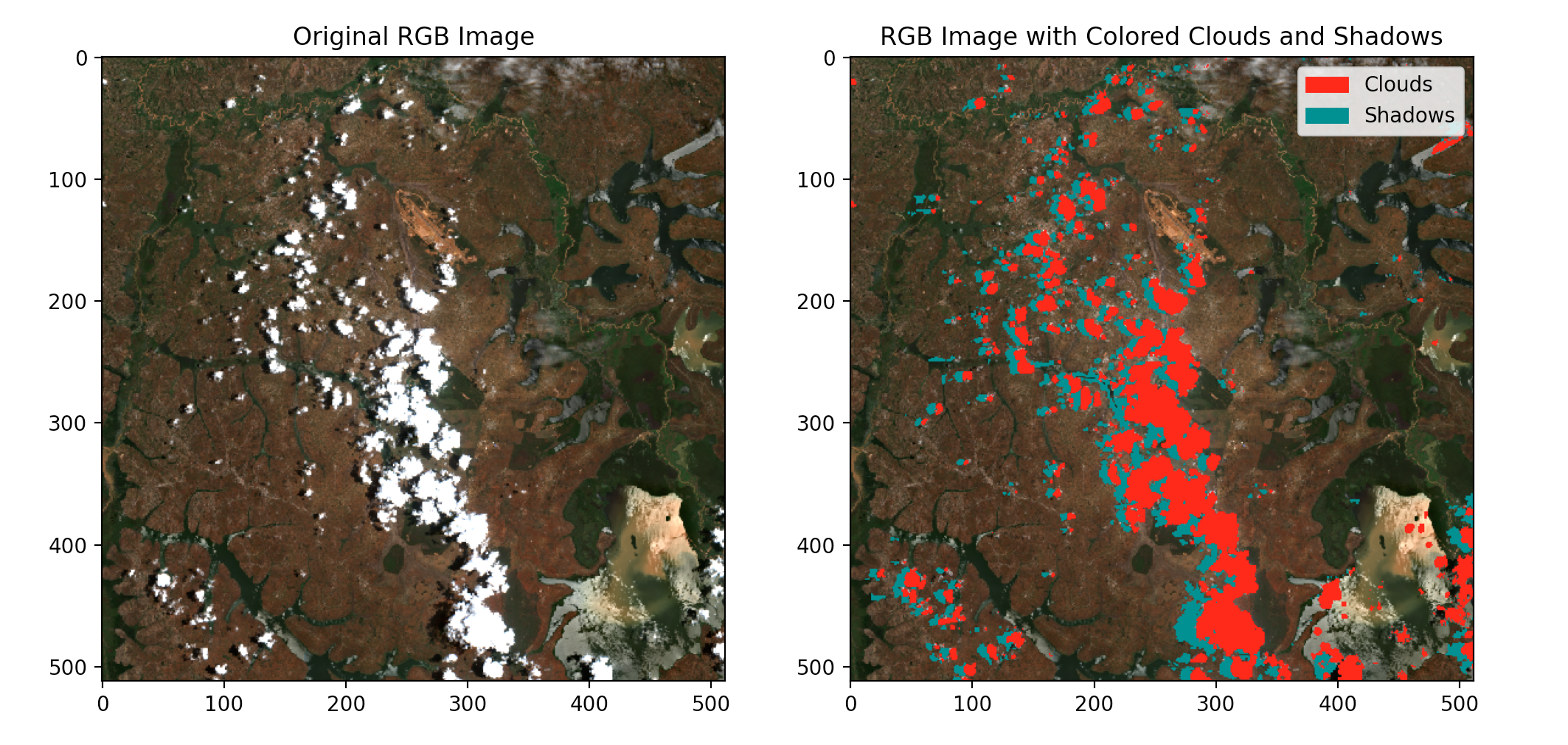
Having the two images, we are ready to As a reminder, we are using Sentinel-2 image as a base due to its advantages over Landsat 8 previously described. The next step is to identify or flag all the cloudy pixels. To do this, the Scene Classification Layer (SCL) of the Sentinel-2 will come in very handy. SCL is a raster layer included in Sentinel-2 Level-2A products, providing information about the classification of each pixel in the image, indicating the dominant type of surface or material present in that pixel. Use the code block below to read and access the SCL.
# Open the Sentinel-2 image


# Function to create colored RGB image with clouds and shadows
def color_clouds_and_shadows(rgb, cloud_mask,shadow_mask):
    colored_rgb = rgb.copy()

    # Define colors for clouds and shadows
    cloud_color = np.array([255, 0, 0])  # Red for clouds
    shadow_color = np.array([0, 128, 128])  # Gray for shadows
    water_color = np.array([0,0,255])
    forest_color = np.array([0,255,0])


    # Use np.where to assign colors based on boolean masks
    colored_rgb[:, cloud_mask] = cloud_color[:, np.newaxis]
    colored_rgb[:, shadow_mask] = shadow_color[:, np.newaxis]
    return colored_rgb


#Read the Sentinel 2 image previously downloaded
with rasterio.open('sentinel2RGB.tif') as src:
    # Read the RGB bands
    rgb = src.read([1,2,3], masked=True)

    # Read the corresponding SCL band
    with rasterio.open("SCL.tif") as scl_src:
        # Read the SCL band
        scl_band = scl_src.read(1, masked=True)

        # Define thresholds for all pixels including cloud and shadow pixels
        '''
        Pixel dictionary for SCL:
        0:No Data (Missing data)
        1:Saturated or defective pixel
        2:Dark features / Shadows
        3:Cloud shadows
        4:Vegetation
        5:Not-vegetated
        6:Water
        7:Unclassified
        8: Cloud medium probability
        9: Cloud high probability
        10: Thin cirrus
        11: Snow or ice

        '''
        cloud_threshold = [8,9]
        shadow_threshold = [3]

        # Define colors for clouds and shadows
        cloud_color = np.array([255, 0, 0])  # Red for clouds
        shadow_color = np.array([0, 128, 128])  # Gray for shadows


        # Create a cloud and shadow mask
        cloud_mask = np.isin(scl_band, cloud_threshold)
        shadow_mask = np.isin(scl_band, shadow_threshold)

        # Visualize pixel distributions of the masks
        plot_pixel_distribution(cloud_mask, 'Cloud Mask Distribution')
        plot_pixel_distribution(shadow_mask, 'Shadow Mask Distribution')

        # Apply the masks to RGB bands using the color_clouds_and_shadows function
        rgb_colored = color_clouds_and_shadows(rgb, cloud_mask,shadow_mask)

        # Visualize the original and colored RGB images
        fig, axes = plt.subplots(1, 2, figsize=(12, 6))
        axes[0].imshow(rgb.transpose(1, 2, 0))
        axes[0].set_title('Original RGB Image')
        #axes[0].legend(["Clouds"])


        axes[1].imshow(rgb_colored.transpose(1, 2, 0))
        axes[1].set_title('RGB Image with Colored Clouds and Shadows')
        axes[1].legend(['Cloud shadows'])

        # Add custom legend
        cloud_patch = Patch(color=cloud_color / 255, label='Clouds')
        shadow_patch = Patch(color=shadow_color / 255, label='Shadows')
        #axes[0].legend(handles=[cloud_patch, shadow_patch])
        axes[1].legend(handles=[cloud_patch, shadow_patch])

        plt.show()
As seen below, we can flag the clouds and their shadows. The red colors show cloudy pixels and the army green shows shadows cast by the clouds.
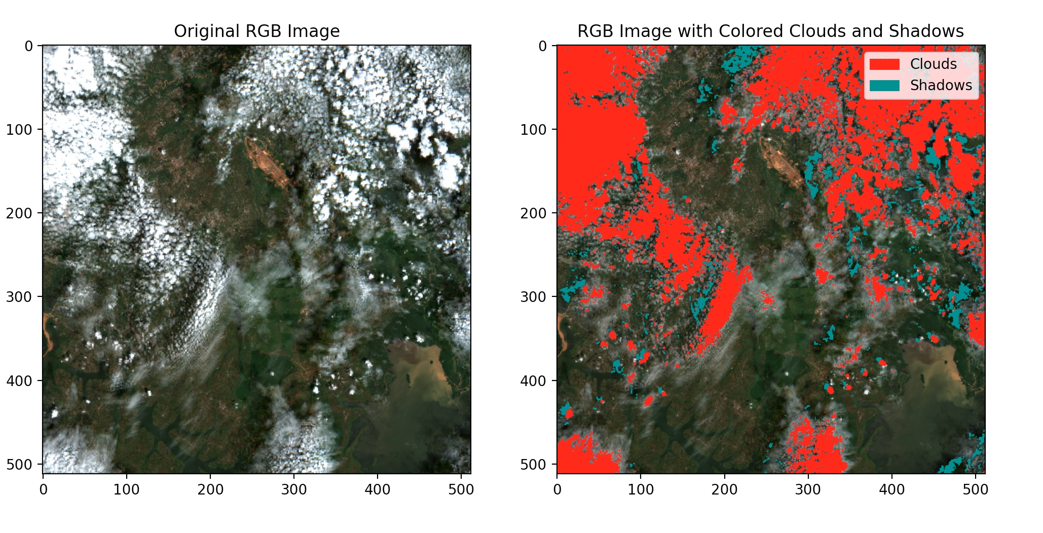
Next, we will replace these pixels(cloudy and shadow pixels) in the sentinel-2 image with near-clear pixels from the Landsat 8 image.
Pixel replacement
# Set the output folder for downloaded images
output_folder = "downloaded_images"

    # Create output folder if it doesn't exist
if not os.path.exists(output_folder):
    os.makedirs(output_folder)


# Function to create colored RGB image with clouds and shadows replaced by Sentinel2  band

def replace_clouds_and_shadow_with_landsat8(rgb, l8, cloud_mask):
    colored_rgb = rgb.copy()


     # Replace cloud pixels in Sentinel 2 RGB with corresponding values from Landsat 8
    colored_rgb[:, cloud_mask] = l8[:, cloud_mask]
    colored_rgb[:, shadow_mask] = l8[:, shadow_mask]


#Save and clip the constructed image to original shapefile
def clip_and_save_image(image_path, shapefile_path, output_folder, output_filename):
    # Read the Sentinel-2 image
    with rasterio.open(image_path) as src:
        # Read the shapefile
        gdf = gpd.read_file(shapefile_path)
        gdf = gdf.set_geometry('geometry')

        # Convert the GeoDataFrame to the same CRS as the Sentinel-2 image
        gdf = gdf.to_crs(src.crs)

        # Use the bounds of the GeoDataFrame as the bounding box for clipping
        bbox = gdf.geometry.total_bounds

        # Perform the clipping
        clipped_image, transform = mask.mask(src, gdf.geometry, crop=True)

        # Update metadata for the clipped image
        out_meta = src.meta
        out_meta.update({"driver": "GTiff",
                         "height": clipped_image.shape[1],
                         "width": clipped_image.shape[2],
                         "transform": transform})

        # Save the clipped image
        output_path = os.path.join(output_folder, output_filename)
        with rasterio.open(output_path, "w", **out_meta) as dest:
            dest.write(clipped_image)


# Open the Sentinel-2 image
with rasterio.open('path/to/sentinel2/RGB.tif') as src:
    # Read the RGB bands
    rgb = src.read([1,2,3], masked=True)
    show(rgb)

    # Open the Landsat 8 image
    with rasterio.open('path to /landsat 8/rgb.tif') as l8_src:
        # Read the Landsat 7 rgb band
        l8_rgb = l8_src.read([1,2,3], masked=True)
        show(l8_rgb)

        # Open the Sentinel-2 SCL band
        with rasterio.open("/path/to/SCL.tif") as scl_src:

            gdf = gpd.read_file(shapefile_path)
            gdf = gdf.set_geometry('geometry')

        # Convert the GeoDataFrame to the same CRS as the Sentinel-2 image
            gdf = gdf.to_crs(src.crs)


                # Read the SCL band
            scl_band = scl_src.read(1, masked=True)
            scl_clip, transform = mask.mask(scl_src, gdf.geometry, crop=True)

                # Update the metadata of the clipped image
            scl_meta = scl_src.meta.copy()
            scl_meta.update({
                    "driver": "GTiff",
                    "height": scl_clip.shape[1],
                    "width": scl_clip.shape[2],
                    "transform": transform
            })

    #return scl_clip, scl_meta

            # Define thresholds for cloud and shadow pixels in SCL band
            cloud_threshold = [8,9]
            shadow_threshold = [3]


            # Create a cloud and shadow mask
            cloud_mask = np.isin(scl_band, cloud_threshold)
            shadow_mask = np.isin(scl_band, shadow_threshold)
            # Apply the replace_clouds_with_sentinel1 function
            rgb_replaced = replace_clouds_and_shadow_with_sentinel1(rgb, l8_rgb,cloud_mask)

            # Visualize the original and modified RGB images
            fig, axes = plt.subplots(1, 2, figsize=(12, 6))
            axes[0].imshow(np.moveaxis(rgb.data, 0, -1))
            axes[0].set_title('Original RGB Image with cloud covers')
            axes[1].imshow(np.moveaxis(rgb_replaced.data, 0, -1))
            axes[1].set_title('RGB Image with Clouds Replaced by Landsat 8 pixels')
            plt.show()
            # Save the composite image with CRS
            output_path = 'downloaded_images/reconstructed_rgb.tif'

            # Define CRS information (change EPSG code according to your needs)

            # Copy georeferencing information from the original Sentinel-2 image
            transform = src.transform
            crs = src.crs

            with rasterio.open(output_path, 'w', driver='GTiff', height=src.height, width=src.width, count=3, dtype=rgb_replaced.dtype, crs=crs, transform=transform) as dst:
                dst.write(rgb_replaced)

        # Save the clipped image with the name of the shapefile
        clip_and_save_image(output_path,shapefile_path, output_folder, f"{os.path.splitext(os.path.basename(shapefile_path))[0]}_clipped.tiff")
 It’s important to note that when performing such replacements, you’ll need to ensure that the Landsat 8 data is properly aligned and resampled to match the resolution and spatial characteristics of the Sentinel-2 imagery. This is achieved by using the georeferencing information from the original Sentinel-2 imagery.
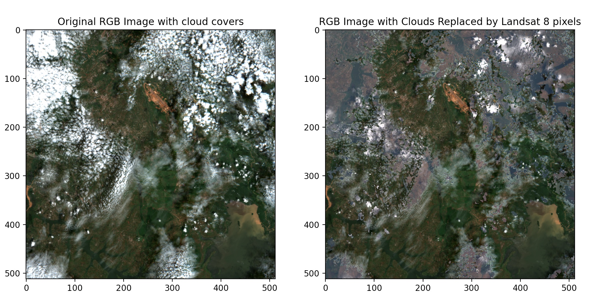
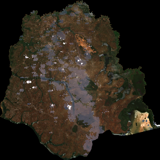
Next, we try the approach again on the same location with different timestamps to demonstrate the reproducibility of the technique. Below are the results.
Finally, we clip the reconstructed image to the location shapefile. This is done to ensure that neighboring pixels are not included in the final image for further predictions and(or) calculations.
Conclusion
To conclude, this tutorial demonstrates the technique of infusing different satellite images into a single one and prepares it as an input for computer visoin downstream . This is especially useful in areas with limited imagery with extremely high cloudy pixels. Another area worth investigating is the possibility of infusing different types of satellite images, i.e optical and SAR image types. If you find this tutorial useful, please leave a comment. Check out my github for the complete code.
Hi. I am Bright Aboh; a data scientist, a climate change researcher and a music lover.